Excel Listdown Top 10 Values in a List

Having looked at extracting a list of unique values we now move on to consider extracting a list of duplicate values. Maybe I can use an IF formula he thinks to himself and decides to give it a go.

How To Get Top Values From A List Or A Table In Excel

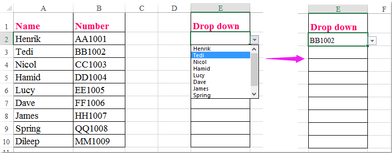
Create a Drop-Down List.

. Tab down to the Source field and click inside this box. To do this task use the HLOOKUP function. Trying to get a list of the top 10 values of R for each of the names in Column A.

Excel UNIQUE function. The UNIQUE function in Excel returns a list of unique values from a range or array. Drop Down List in Excel is mainly used in an organization like data entry and medical transcription data dashboards to choose and update the validation data in an easier way from the Drop Down list.

Howto set up Drop Down list in Excel. Must know your top 10 values what they mean for you which ones are most important and which ones youre not living up to. You would notice that the unique product name list is extracted in column E.

For more information see HLOOKUP function. Values basically define whats most important for you in life and if youre not making that a practice you will not be happy or successful long-term. Move your cursor outside of this dialog window and select the lists spreadsheet from the workbook tabs at the bottom of the screen.

Look up values horizontally in a list by using an. Go to Data ribbon and click on Validation. The data added to a drop-down list can be located on either the same worksheet as the list on a different worksheet in the same workbook or in a completely different Excel workbook.

Type this formula into Cell E2 and press Ctrl Shift Enter keys to change it as Array formula. I have copied my original list to a second column and then with the function of Excel remove duplicates I could find the list of unique values. A simple way to do this would be to combine the Index and Match functions like this.

In excel drop-down list is a useful feature that enables us to choose the value from the list box. Text numbers dates times etc. Select the data list excluding the list label and click Kutools Select Select Duplicate Unique Cells.

See an example below. Trying my best to get this down and translate it to my problem. However after several failed attempts he decides to.

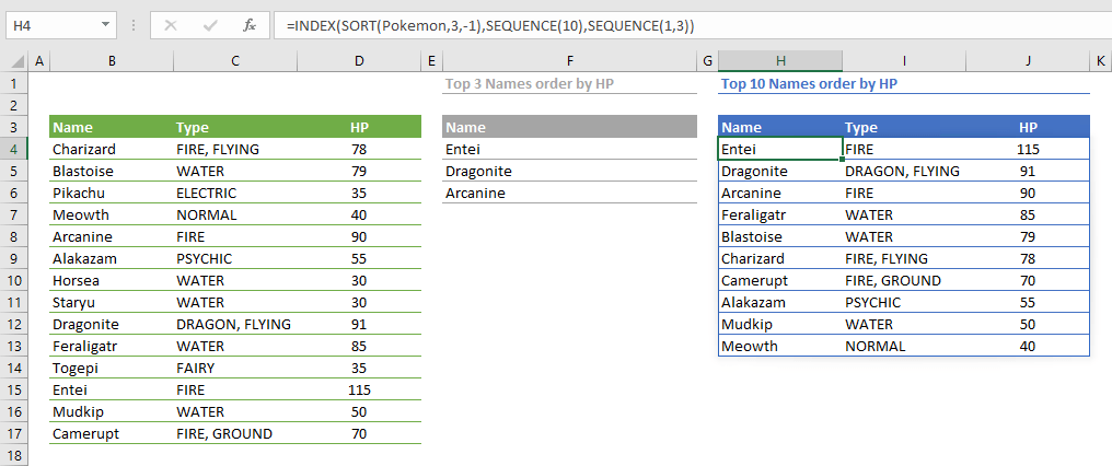
In this example we are also going to be using the INDEX function to display only n number of values. Column N is a binary choice either 0 or 1 and column R is a calculated value. In this tutorial were using a list of cookie types.

Formulas are the key to getting things done in Excel. The formula in Cell D3 is so long that it is included on two lines below but you can have it on a single line within Excel. To follow along enter the data in columns D and E shown in the image below.

Look up values horizontally in a list by using an exact match. Set up List as allowed values and enter A1A6 as Source see below picture Done. Here is the list of Top 10 Basic Formulas Functions in Excel.

Get top n values from a list. Here is the formula that it will extract the unique distinct product name list based on month value. Now go the cell where you want to validation drop down to appear.

If you already made a table with the drop-down entries click in the Source box and then click and drag the cells that contain those entries. The result is a dynamic array that automatically spills into the neighboring cells vertically or horizontally. On the Settings tab in the Allow box click List.

In the Microsoft Visual Basic for Applications window click Insert. The function is categorized under Dynamic Arrays functions. Lets start with the SORT function.

First set up a list of valid values in range of cells. In this accelerated training youll learn how to use formulas to manipulate text work with dates and times lookup values with VLOOKUP and INDEX MATCH count and sum with criteria dynamically rank values and create dynamic ranges. Now you can see the drop-down in your cell.

Extract a list of duplicate values. I have a spread sheet where column A is a list of names alphabetical from row 4 to row 1200 with only 8 different names. Nathan is working on a spreadsheet that contains a list of car models and owners.

Click the top left cell of the range and then drag to the bottom right cell. Create a Unique List in Excel based on Criteria. However do not include the header cell.

Highlight the range of doctorsthat is A2 through A11. He needs to create a unique list of owners per car. Hence Excel Drop Down List saves the time.

Say your valid list of entries is in A1A6. It works with any data type. The drag the AutoFill handle until you get the NA value.

Select all the rows including the column headers in the list you want to filter. Go to the Data tab on the Ribbon then click Data Validation. Copied from Microsoft Office Website.

You can also extract a list of unique values dynamically from a column range with the following VBA code. From the Settings tab choose List from the list box. Press Alt F11 keys simultaneously to open the Microsoft Visual Basic for Applications window.

INDEX AAMATCH E1BB0 This assumes your client names are in column A Revenue is in column B and the the large revenue you are looking up is in cell E1 Additionally this simple approach will return the first client name with the large revenue and. In the Select Duplicate Unique Cells dialog check Unique values only or All unique Including 1st duplicates box as your need and click Ok a dialog pops up to tell you how many rows are selected click OK to. INDEX function can get values from a given positionAlthough it is designed to get values from a single cell we will enhance it to get rows or columns with the help of the SEQUENCE function.

HLOOKUP looks up the Sales column and returns the value from row 5 in the specified range.

Dependent Drop Down List For Multiple Rows Using Excel Dynamic Arrays Ablebits Com

How To Create Drop Down List But Show Different Values In Excel

How To Get Top Values From A List Or A Table In Excel